ECON 0150 | Economic Data Analysis
Dr. Taylor Weidman
taylorjweidman@pitt.edu | 4702 Posvar Hall
ECON 0150 | Economic Data Analysis
Dr. Taylor Weidman
taylorjweidman@pitt.edu | 4702 Posvar Hall
ECON 0150 | Economic Data Analysis
Taylor
taylorjweidman@pitt.edu | 4702 Posvar Hall
ECON 0150 | Economic Dada Analysis
Taylor
taylorjweidman@pitt.edu | 4702 Posvar Hall
ECON 0150 | Economic Dada Analysis
What is economic dada analysis?
What is economic data analysis?
Economists use data to build models and inform decisions.
Describing the landscape of economics
- Have incomes risen in the last year?
- How has unemployment changed?
- Has the racial wealth gap narrowed?
Distinguishing between economic theories
- Do voters with neighbors of the same party vote more?
- Does the gender of a Lyft driver impact rates of tipping?
- Is cooperation higher in ‘easier’ repeated prisoner’s dilemmas?
Course Goals
Skillset 1. Summarize data (tables and figures).
Skillset 2: Build and interpret models (general linear model).
Skillset 3: Communicate findings (writting and presentations).
Goal: I want you to be able to build appropriate statistical models for new problems and interpret their results.
Course Structure
Part 1: Exploring Variables
Part 2: Exploring Relationships
Part 3: Univariate General Linear Model
Part 4: Bivariate General Linear Model
Part 5: Multivariate General Linear Model
Part 6: Communicating with Data
Part 1: Exploring Variables
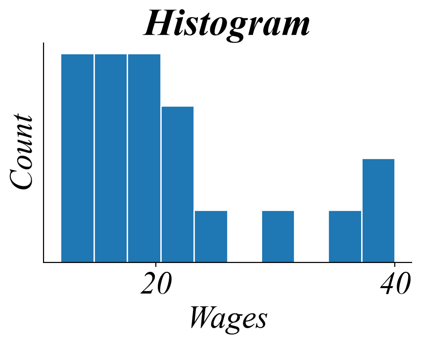
Example: Analyzing a dataset of wages.
| 12 |
8 |
| 13 |
10 |
| 14 |
10 |
| 14 |
11 |
| 15 |
12 |
Part 2: Exploring Relationships EDA
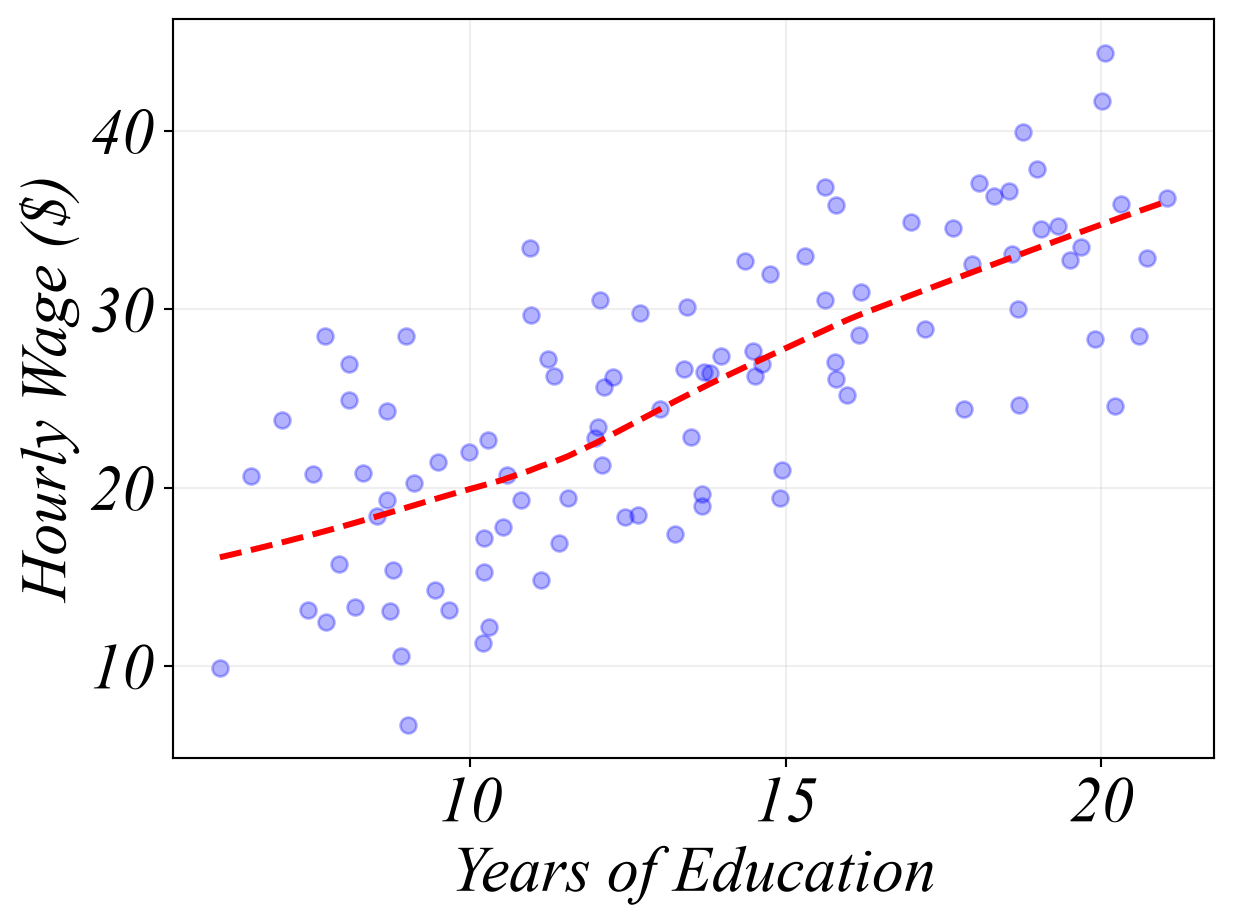
Example: Exploring a relationship - education and wages.
| 0 |
14 |
10 |
| 1 |
15 |
12 |
| 2 |
16 |
12 |
| 3 |
18 |
13 |
| 4 |
18 |
14 |
| 5 |
20 |
14 |
| 6 |
22 |
15 |
Part 3: Univariate Regression
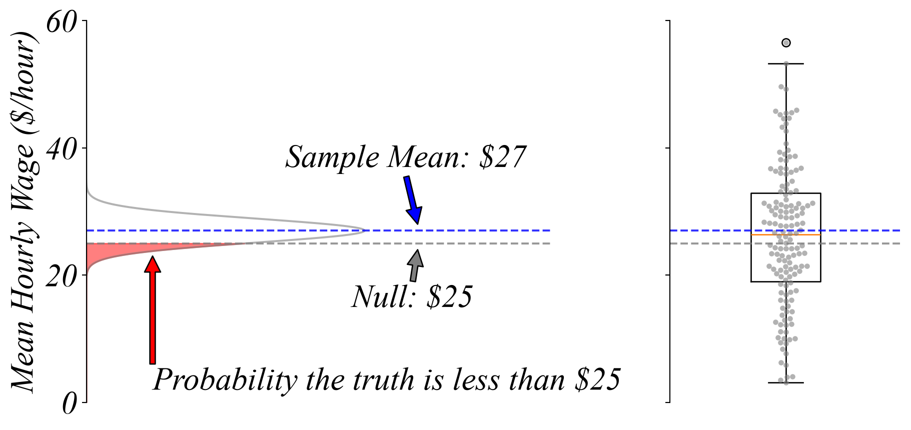
Example: Is the difference from $25 a real pattern or just noise?
Part 4: Bivariate Regression
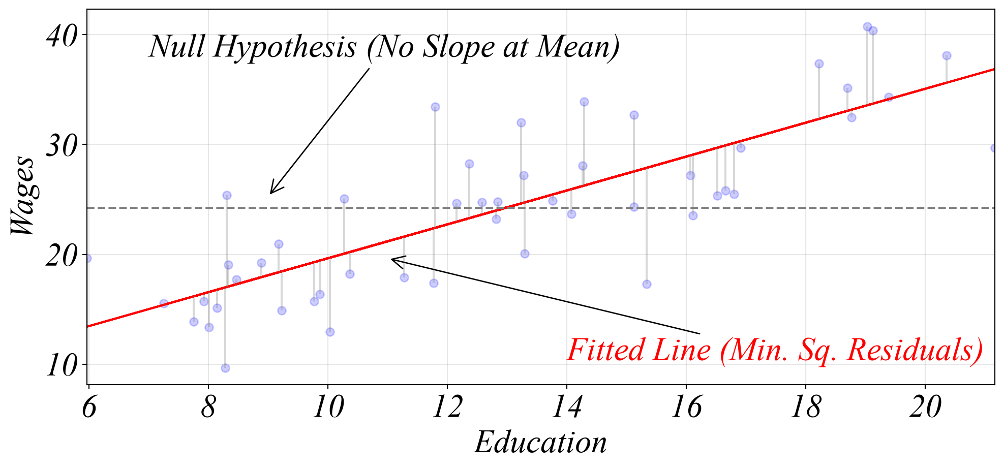
Example: Is the positive slope a real pattern or just noise?
Part 5: Multivariate Regression
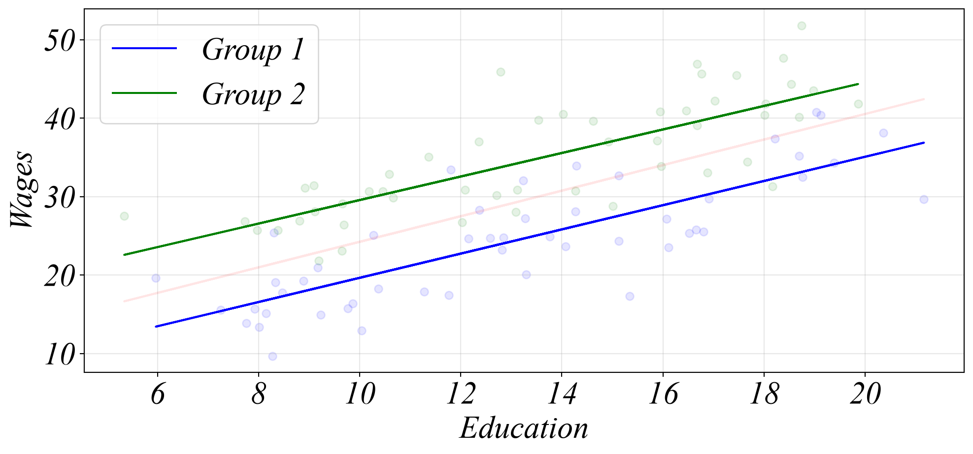
Example: Do different groups have different relationships?
Part 6: Communicating with Data
Examples: Some student work from last semester!
Your Work
Exercises (10%)
- Together in class; lowest 3 dropped.
Homework (10%)
- Fridays by 5PM; lowest 3 dropped.
- No-questions-asked extensions through Sunday at Midnight.
MiniExams (1 × 15% + 1 × 15% + 1 × 10% + 1 × 5% + 1 × 5% = 50%)
- Roughly every two weeks; beginning of class
- Open-book, open-note (no electronics).
Your Work
Final Project (30%)
- One small project per part.
- Presentation + paper at the end of the semester.
- Demonstrate full analysis from start to finish.
Policies
Email Policy:
- Response may take up to 1-2 days.
- Be concise with your questions.
- My email is off evenings and weekends.
AI Policy:
- Encouraged as a learning and coding tool :)
- Your work must be your own.
- Cite your source.
Looking Ahead
First Homework:
- Due (next) Friday at 5PM on Gradescope
First MiniExam:
- First class of Week 4 during the first 20 minutes.
Getting Set Up
Excel:
- Free for students through Pitt’s institutional access
Python:
ECON 0150 | Economic Data Analysis
Block 0. Why does economic data analysis matter?
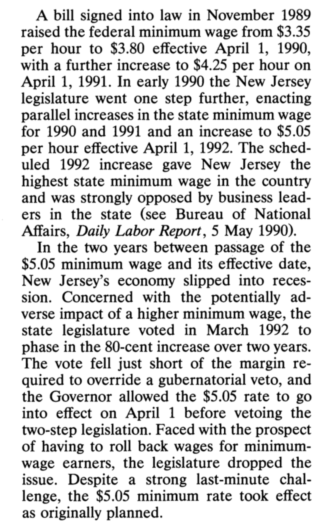
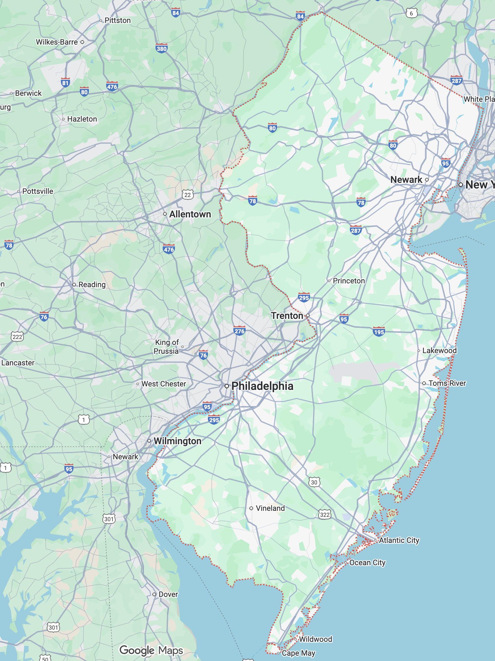
New Jersey, 1992
| March 1992 |
$4.25 |
$4.25 |
| April 1, 1992 |
$5.05 |
$4.25 |
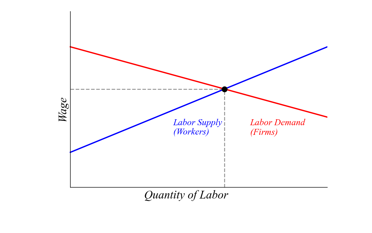
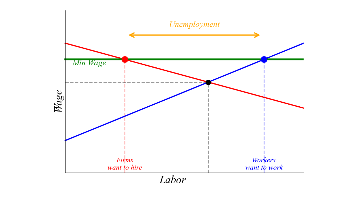
What happens to employment?
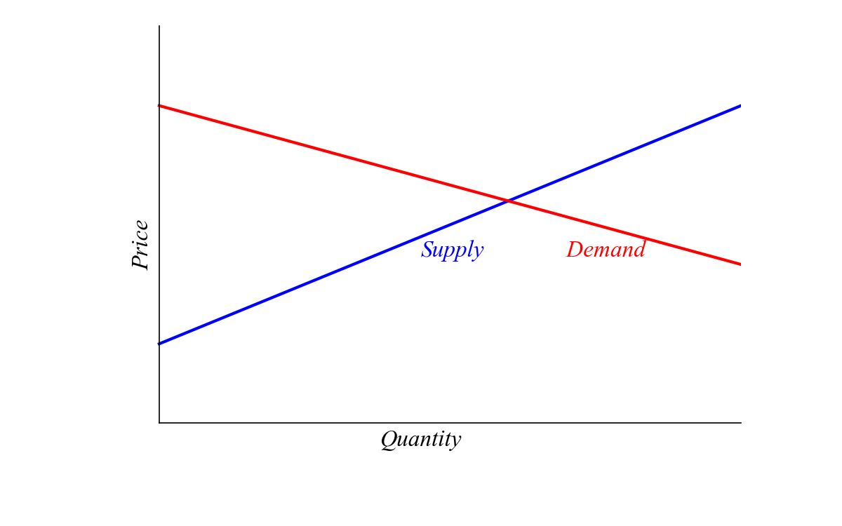
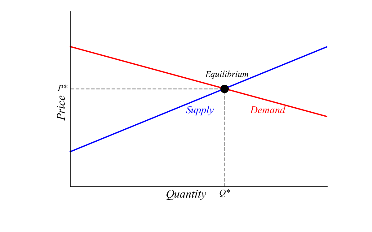
Economic Theory
![]()
Economic Theory
![]()
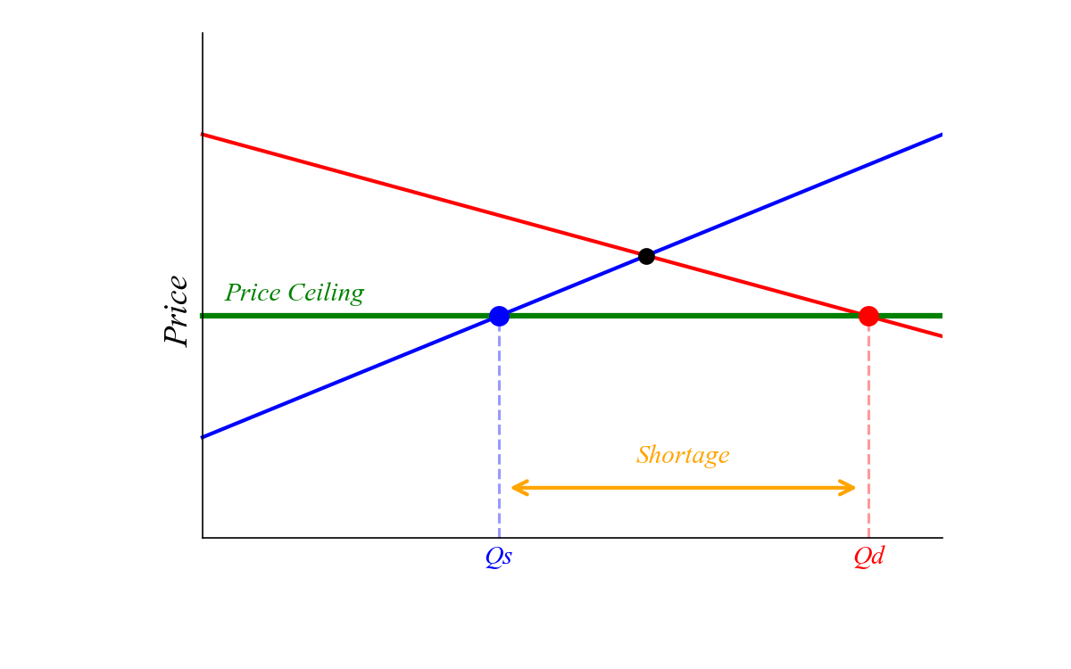
Economic Theory
![]()
Economic Theory
![]()
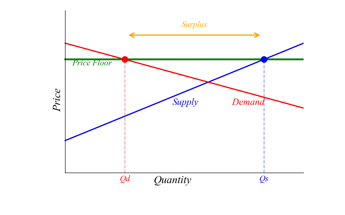
Economic Theory
![]()
Economic Theory
![]()
Card and Krueger

David Card

Alan Krueger
Data
| Timing |
Feb-Mar 1992 |
Nov-Dec 1992 |
| Policy |
Before increase |
After increase |
| Stores |
410 |
399 |
Burger King, KFC, Wendy’s, Roy Rogers in NJ and eastern PA
Data
| Stores surveyed |
331 |
79 |
| FTE employment |
20.4 |
23.3 |
| Starting wage |
$4.61 |
$4.63 |
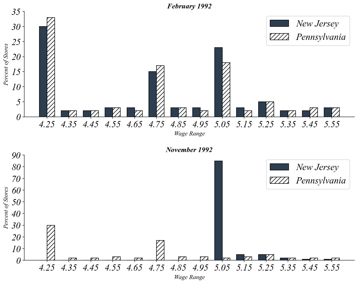
| Wage = $4.25 |
30.5% |
32.9% |
Data
![]()
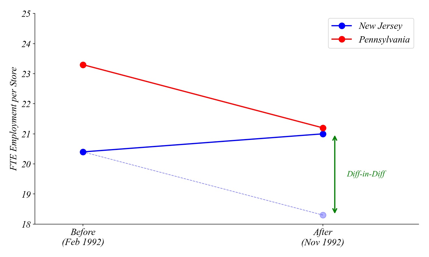
Analysis
![]()
Results
| Before |
23.33 |
20.44 |
-2.89 |
| After |
21.17 |
21.03 |
-0.14 |
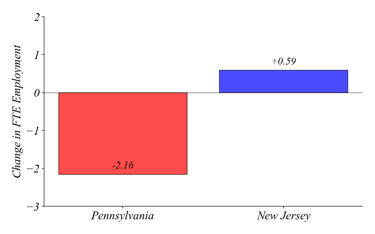
| Change |
-2.16 |
+0.59 |
+2.76 |
Results
![]()
Theory vs. Evidence
Theory prediction
- higher minimum wage → lower employment
Data showed
- no decrease in employment
“Contrary to the central prediction of the textbook model… we find no evidence that the rise in New Jersey’s minimum wage reduced employment.”
Card and Krueger (1994)
Let’s learn how to do this kind of analysis.
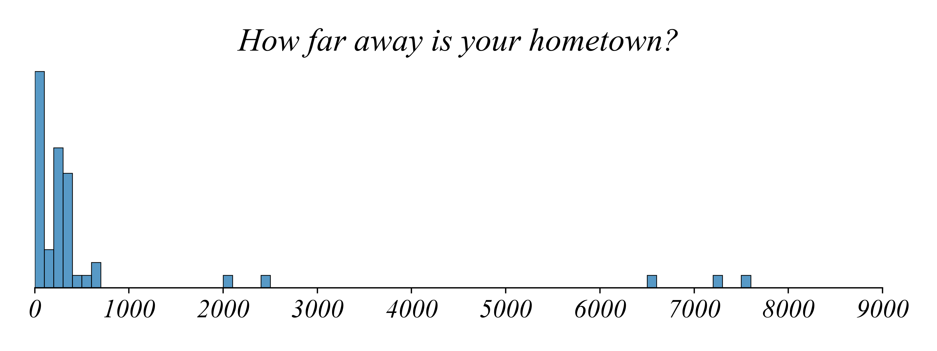
Where are students coming from?
Where are students coming from?
![]()
> quite a few people come internationally :)
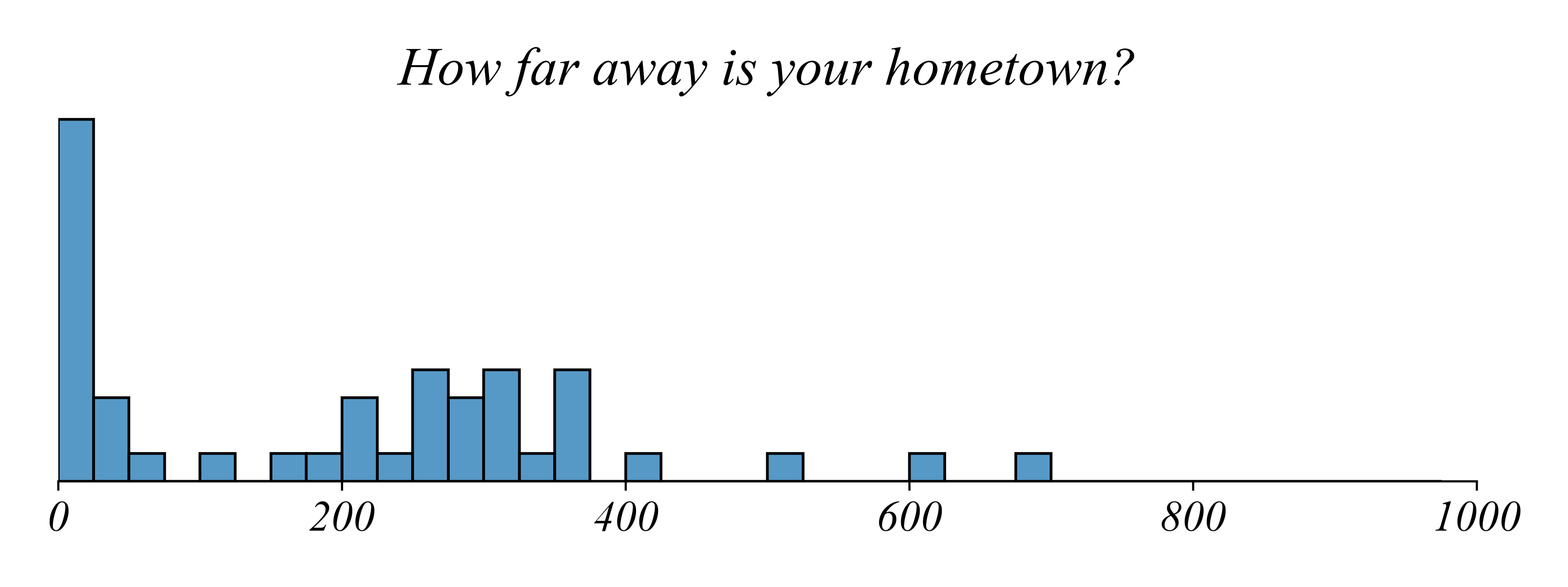
> lets zoom in a bit to see more details about closer distances
Where are students coming from?
![]()
> many from Pittsburgh and the Philly area
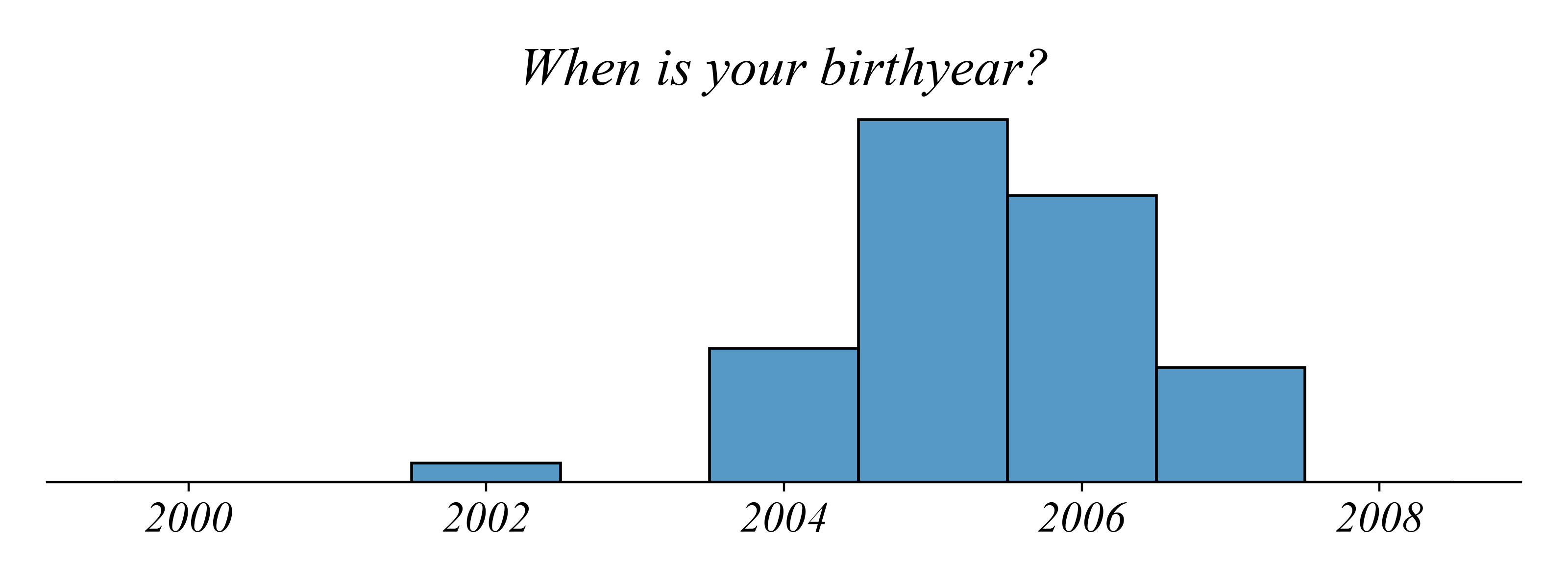
When were students born?
![]()
> the most common birthyear was 2005
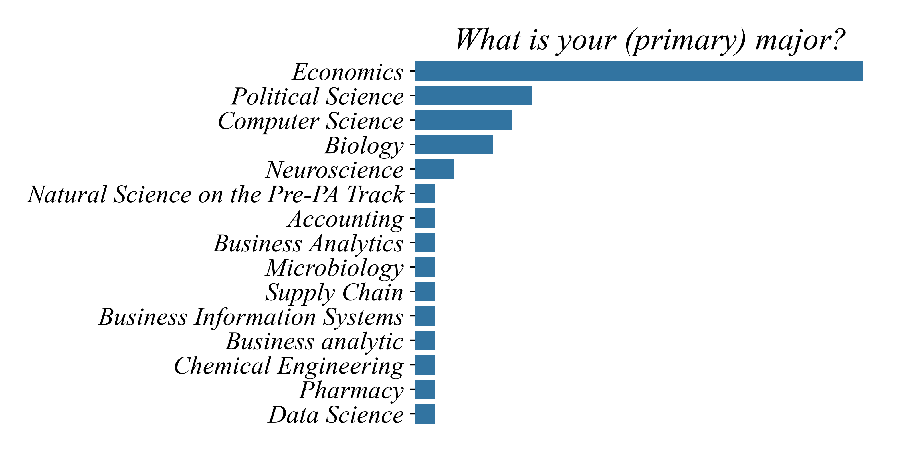
What are students majors?
What are students majors?
![]()
> most are Econ and many not on my limited list
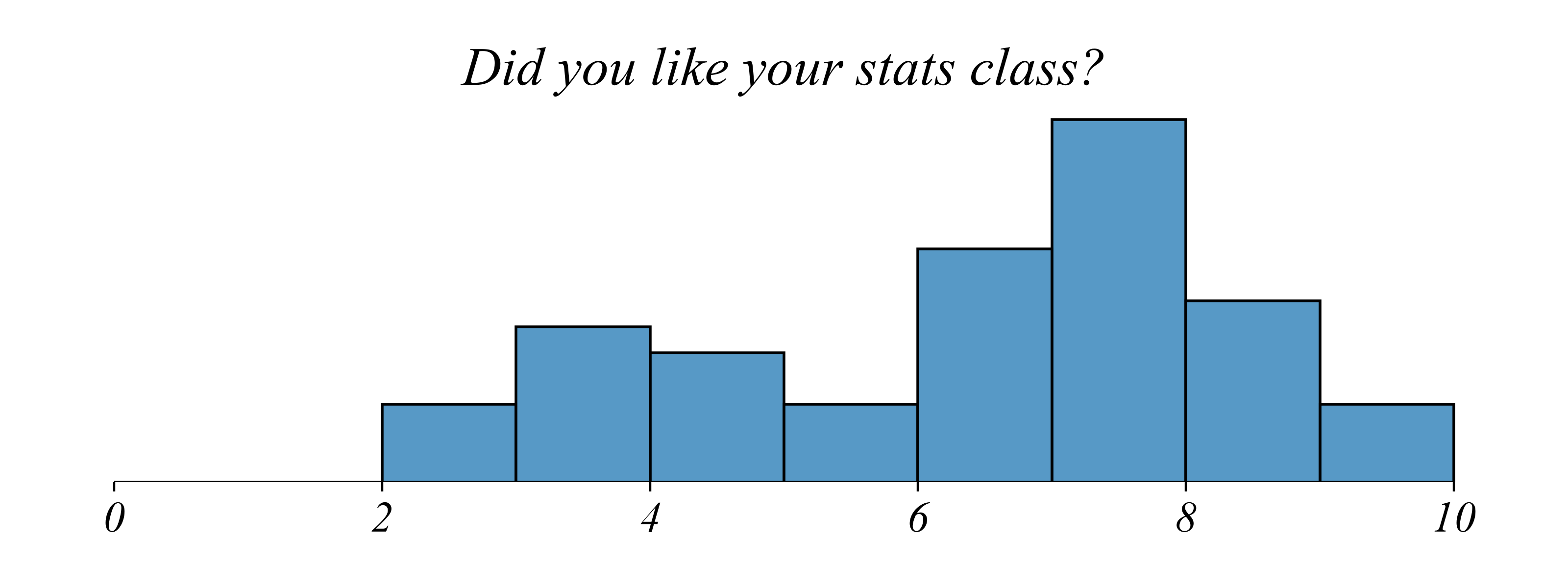
Did you like your stats class?
Did you like your stats class?
![]()
> most generally liked it; some did not
What is Data?
\[x \sim F\]
- \(x\) = what we observe (our data)
- \(F\) = what generated it (the random variable)
We have \(x\). We care about \(F\).
Two skills:
- Description (Parts 1 - 2): Summarize \(x\).
- Inference (Parts 3 - 5): Learn about \(F\) from \(x\).
How Do We Organize Data?
We write \(x_{it}\) where:
- i (unordered) indexes entities (eg. people, firms, countries)
- t (ordered) indexes time (eg. days, months, years)
This distinguishes substantive variables (what we measure) from index variables (how we organize).
Dimensions of Data
Data Structure (\(i\),\(t\))
- Cross-sectional
- Timeseries
- Panel
Number of Variables (\(n\))
- Univariate (n=1)
- Bivariate (n=2)
- Multivariate (n>2)
Data Structures
| Cross-section |
Entity (i) |
Household incomes in 2024 |
| Time series |
Time (t) |
Average US income from 1950–2024 |
| Panel |
Both (i and t) |
Income across households, 1950–2024 |
Variable Types
| Categorical |
Binary |
Two categories |
Employed (YES/NO) |
|
Nominal |
Unordered |
Blood type (A, B, AB, O) |
|
Ordinal |
Ordered |
Education (HS, BA, MA, PhD) |
| Numerical |
Discrete |
Countable |
Number of children |
|
Continuous |
Real numbers |
Household income |
How We Work with Data
- SELECT: What does our data contain?
- TRANSFORM: How do we change the data to make it more useful?
- ENCODE: How do we turn values into visual elements?
Course Progression
| 0 |
Framework |
What tools do we need? |
| 1 |
Variables |
What does this variable look like? |
| 2 |
Relationships |
How do these variables relate? |
| 3 |
Univariate OLS |
What can we infer about the population? |
| 4 |
Bivariate OLS |
How does y change with x? |
| 5 |
Multivariate OLS |
How does y change with x, controlling for z? |
How Each Class Works
| In class |
New Concepts |
Learn core ideas |
| During class |
Exercise |
Guided practice with support |
| After class |
Homework |
Independent practice |
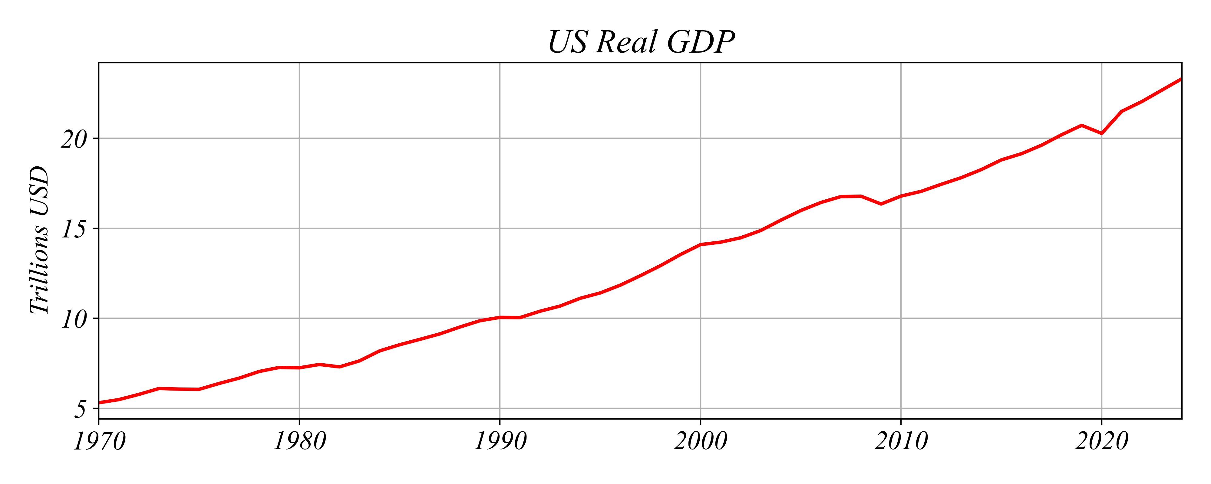
Exercise 0 | Diagram Data
| 1970 |
5.316 |
| 1971 |
5.491 |
| 1972 |
5.780 |
| 1973 |
6.106 |
| … |
… |
Index: \(t\) (Year)
Structure: Time series
Variable: Continuous
N Variables: Univariate
Exercise 0 | Diagram Data
![]()
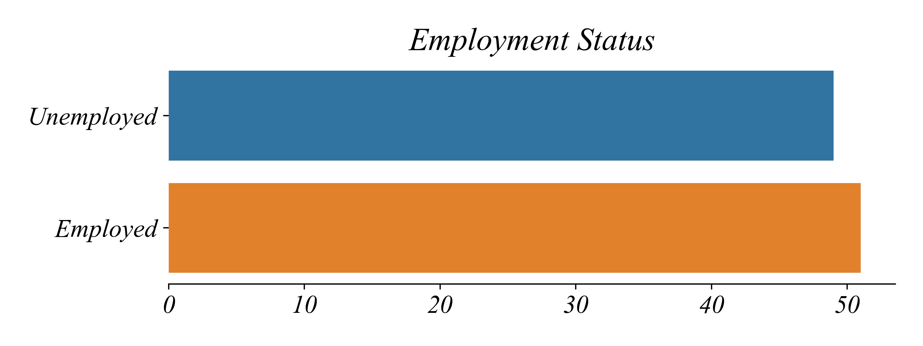
Exercise 0 | Diagram Data
| D001 |
Unemployed |
| D002 |
Employed |
| D003 |
Employed |
| D004 |
Employed |
| … |
… |
Index: \(i\) (Household)
Structure: Cross-sectional
Variable: Binary
N Variables: Univariate
Exercise 0 | Diagram Data
![]()
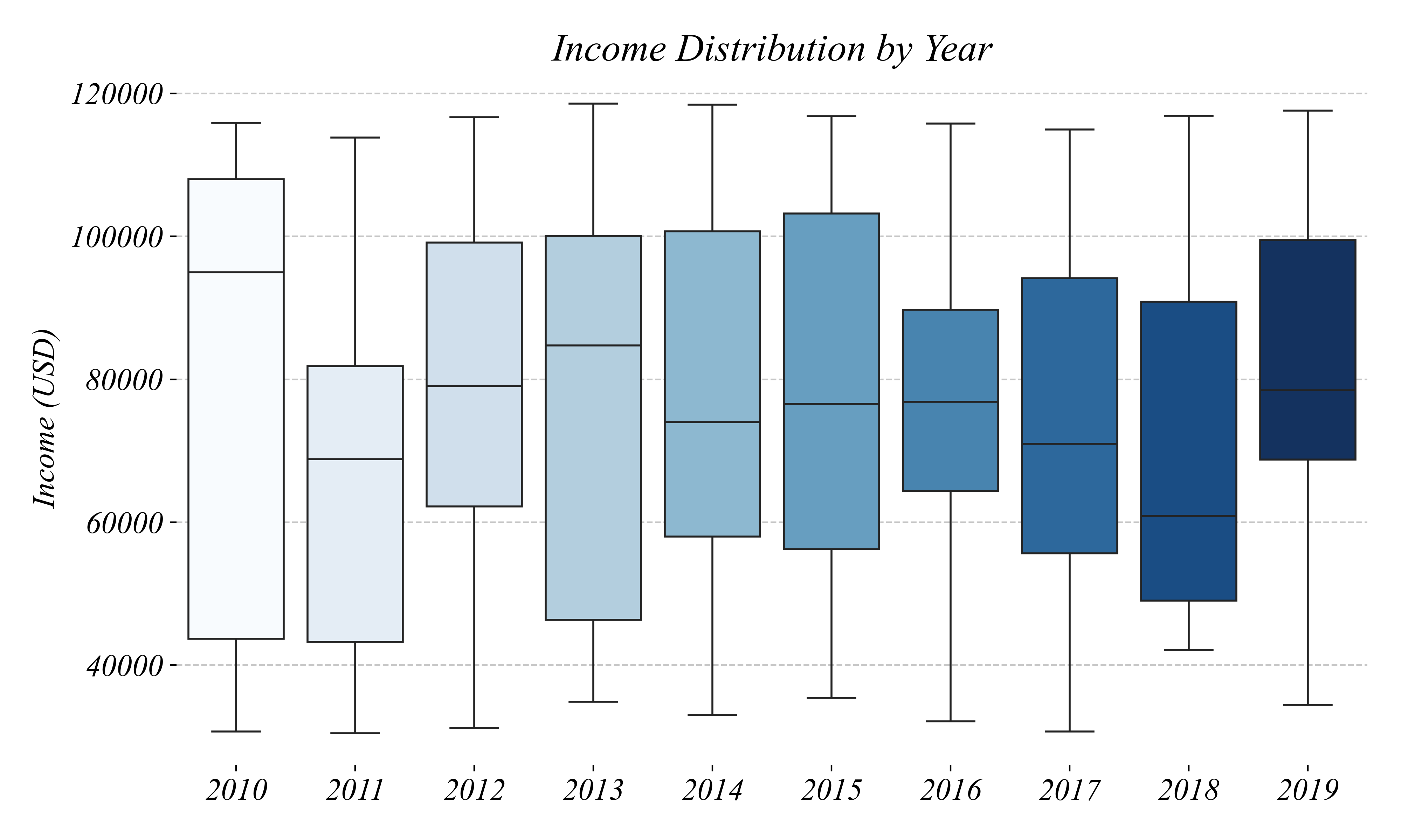
Exercise 0 | Diagram Data
| H001 |
2010 |
34,610 |
6,157 |
| H001 |
2011 |
45,560 |
2,506 |
| H001 |
2012 |
83,698 |
8,789 |
| H002 |
2010 |
52,341 |
4,123 |
| … |
… |
… |
… |
Index: \(i\) (Household), \(t\) (Year)
Structure: Panel
Variable: Continuous
N Variables: Bivariate
Exercise 0 | Diagram Data
![]()
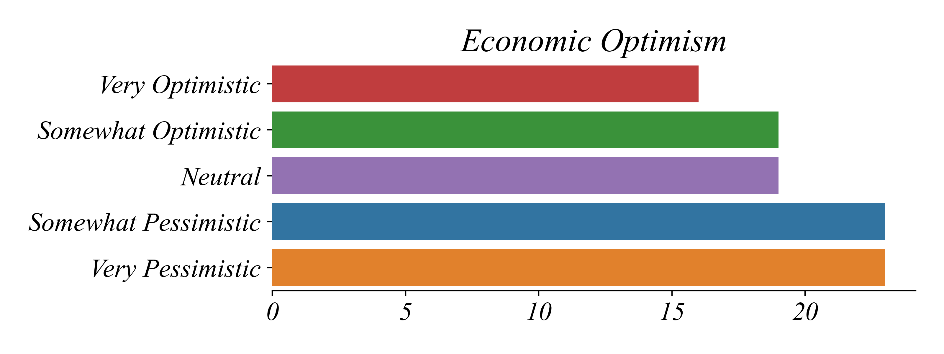
Exercise 0 | Diagram Data
| B001 |
Somewhat Pessimistic |
| B002 |
Very Pessimistic |
| B003 |
Somewhat Optimistic |
| B004 |
Very Optimistic |
| … |
… |
Index: \(i\) (Person)
Structure: Cross-sectional
Variable: Ordinal
N Variables: Univariate
Exercise 0 | Diagram Data
![]()
Exercise 0 | Diagram Data
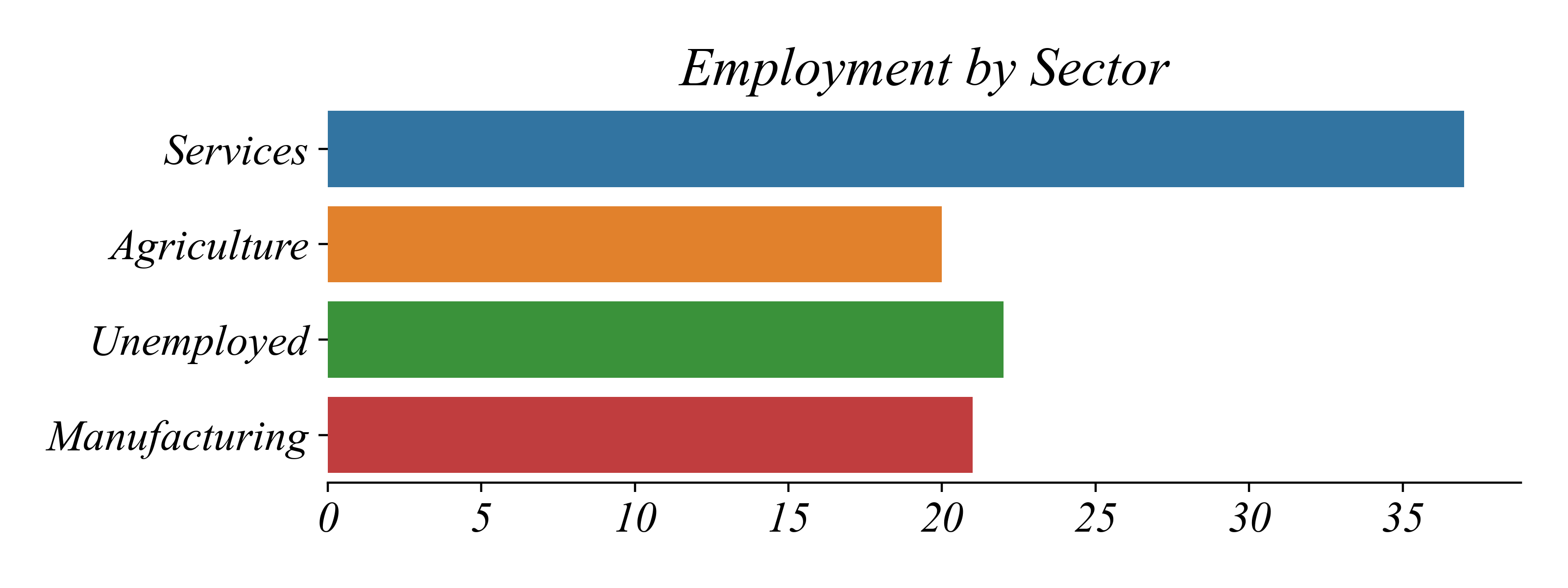
| A001 |
Services |
| A002 |
Agriculture |
| A003 |
Unemployed |
| A004 |
Manufacturing |
| … |
… |
Index: \(i\) (Person)
Structure: Cross-sectional
Variable: Nominal
N Variables: Univariate
Exercise 0 | Diagram Data
![]()